Spectral Modeling in Fluorescence Microscopy
Introduction to Fluorescence Microscopy
Fluorescence microscopy is a ubiquitous and continuously evolving technique which permits one to peer into the biological world at the micron length scale and beyond, allowing direct access into the spatial location and behavior of small molecules at the cellular level. This level of performance can be achieved only through careful instrument design and the use of high quality and high-performance optical components, such as optical filters. Optical filters transmit and block (via reflection) light over specific, well-defined spectral ranges. Filters with poor transmission, edge steepness, and blocking offer limited performance and, in the case of fluorescence microscopy, can result in the acquisition of images with poor contrast, thus limiting the ability to reveal the secrets of the subcellular world. To avoid this limitation, microscopists have been rapidly switching to modern hard-coated thin-film interference filters. Given the critical role optical filters play in fluorescence microscopy, it is important to understand how such filters transmit both the desired fluorescence signal as well as the undesired background light (i.e., optical “noise”).
Two critical performance criteria for any optical system that generates, captures, and records fluorescence light are the level of desired light signal detected and the level of undesired light or optical noise that originates from, for example, stray light and background fluorescence. Knowledge of the power levels of each of these permits the computation of the optical signal-to-noise ratio (SNR), thus making it possible to quantify the microscope performance. A simple definition of the optical SNR is
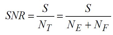
(1)
where S is total detected (desired) fluorescence signal and NT the total (undesired) optical noise, which includes excitation light noise (NE) and fluorescence noise (NF) contributions. The SNR provides a reasonable measure of the overall system performance, which typically correlates well with an observer’s perception of the fidelity of a fluorescence image. Note that for viewing by eye only, the optical noise completely describes the performance. However, for digital imaging with a CCD or CMOS camera, there are additional electronic noise contributions that must be taken into account, including signal-independent contributions (often called “dark current”) and signal-dependent contributions (such as “shot noise,” which can be appreciable for very low-light-level detection). In this article we restrict our discussion to optical noise sources, as there are numerous excellent references that cover electronic noise considerations [1 – 4].
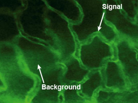
Figure 1: Example of background fluorescence observed on a sample of mouse prostate vasculature (blood vessels). The image contrast is provided by spectrally integrating the fluorescence emission from FITC conjugated to target CD41 marker (mouse) antibodies. The background signal is due to NAD(P)H. Image acquired using a standard epi-fluorescence microscope.
Optical noise manifests itself as a decrease in image contrast between regions of interest (ROIs) where the target fluorophore, which emits fluorescence photons under the appropriate excitation, is located and the surrounding region where no target fluorophore is present. For the case of fluorescence microscopy, images with SNR > 20 are considered acceptable, with values of SNR > 40 desired. In situations where the SNR is less than about 20, careful consideration is required to fully assess and understand the origin of the reduced image contrast. Figure 1 demonstrates a fluorescence image of FITC conjugated to target CD41 marker (mouse) antibodies. What is clear from this image is the effect that unwanted light signals (i.e., optical noise) have on image contrast. From this simple example, it is evident that choice of the correct filters that match and transmit the spectral characteristics of the target fluorophore(s) and at the same time block unwanted light, working in unison with the entire optical system, is critical for recording fluorescence microscopy images with high contrast and high brightness.
Modeling Fluorescence Microscopy
Fluorescence microscopes are typically arranged in the epifluorescence configuration, as illustrated in Figure 2 (left). Excitation light, typically from either a high power arc lamp or a laser, passes through a bandpass “exciter” filter, is reflected by a “dichroic beamsplitter,” and is focused at the sample surface using a microscope objective. In the epifluorescence configuration the microscope objective has two important functions, acting as both the condenser to focus the excitation light onto the sample and the objective to collect the emitted fluorescence. After passing through the objective and the beamsplitter, the emitted fluorescence is transmitted through a second bandpass “emitter” filter and is then imaged either via an eyepiece into the eye of a visual observer or onto a camera. Also shown in Figure 2 (right) are spectral profiles that represent spectral characteristics of those optical components that control the transmission and blocking of light, as well as the absorption and emission spectra of a target fluorophore.
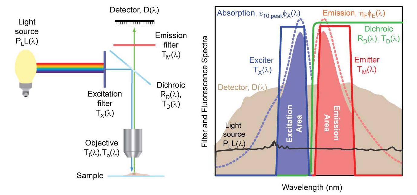
Figure 2: A schematic of an epi-fluorescence microscope configuration based on optical filters (left), and examples of absorption and emission spectra for a target fluorophore and transmission spectra for a set of optical filters (right). The light source (black) is a xenon arc lamp with the detector response profile (brown) representing a typical (cooled) CCD camera. See text and Appendix B for additional details.
In microscopy, signal strength is typically described by intensity. However, for a given power carried by a beam of light, the intensity level can be different depending upon the cross-sectional area of the beam. Therefore, from a system design perspective, we use the power of a beam (rather than intensity level) as a fundamental variable for evaluating the optical performance of the system. Note that it is assumed in the following calculation that all of the light signal is carried in the form of a “beam” of light, where the beam refers to a ray-bundle with a finite cross-section. It is also assumed that the transverse dimensions of all the system components (lenses, filters, sample, detector, etc.) exceed the transverse dimensions of the beam. Further, we assume that none of the optical elements, such as filters and lenses, absorb light and therefore they only transmit or reflect light. With these assumptions the signal and noise can be accurately traced through the system in the form of optical power.
Light Absorption and Fluorescence Emission
Fluorescence emission that results from the absorption of light from an excitation source depends on the absorption and emission characteristics of the target fluorophore, its concentration in the sample, and the optical path length (or characteristic absorption depth, d) of the sample.
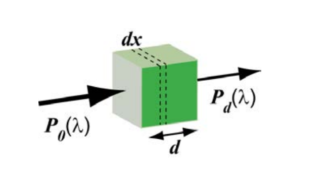
Figure 3: Phenomenological description of power absorption according to Beer-Lambert law. P0(λ) is the power of the incident light, Pd(λ) is the wavelength-dependent power of light emerging from a slab of thickness d. Note that dx is the variable of integration in Eq.(2).
The absorption of light by a fluorophore (or more generically a system of molecules, such as a concentration of fluorophores within a cell) is readily understood on the basis of the Beer-Lambert law [5], which can be derived as follows (Fig. 3):
(2)
where P(λ) is the wavelength-dependent power of light, σ(λ) is the molecular absorption cross section (dimensions cm2), and ρ is the number density of molecules (dimensions molecules/cm3). Even though the molecular absorption cross section σ(λ) has units of area, it does not necessarily denote the physical cross-section area of the fluorophore molecule; rather this term denotes an effective cross-sectional area of the molecule which describes the probability of absorbing a photon of a particular wavelength. Solving the above equation with the boundary conditions of P(λ)=P0(λ) at x=0, and P(λ)=Pd(λ) at x = d, yields the more familiar exponential form of the Beer-Lambert law:
(3)
where Pd(λ) is the wavelength-dependent power of light emerging from a slab of thickness d, and P0(λ) is the power of the incident light.
While the Beer-Lambert law in the form of Equation (3) provides a phenomenologically pleasing picture for the absorption process, the properties of the absorbing fluorophores are more easily characterized by the extinction coefficient ε(λ) (dimensions cm2/mole = M–1cm–1) and the molar concentration of target fluorophore c (dimensions M = molar = moles / liter = 10–3 moles / cm3). These quantities are related to σ(λ) and ρ via the relationship [5]
(4)
Note that since c/ρ = 103/N, where N is Avogadro’s number, σ and ε are directly related by σ = 1.66×10⁻²¹ ε. Using Equation (4), we can now rewrite (2) as
(5)
Equation (5) gives the light power emerging from a slab of thickness d containing a homogeneous molar concentration c of fluorophore with extinction coefficient ε.
We can now consider the total amount of light absorbed by some medium containing a concentration of fluorophores. Mathematically, the absorbed light power can be written as
(6)
where P0(λ) and Pd(λ) are as defined above. Upon substituting for Pd(λ) and considering the case of low fluorophore concentration, the absorbed light power Pabs(λ) can be approximated by
(7)
Fluorophore absorption properties are commonly characterized by a parameter called the “decadic molar extinction coefficient,” ε10(λ) (or decadic molar absorption coefficient, DMAC). This quantity is related to ε(λ) according to
(8)
or
(9)
The extinction coefficient may then be related to the normalized fluorophore absorption spectral profile φΑ(λ) via the following relationship

(10)
where ε10,peak represents the maximum value of the decadic molar extinction coefficient and is a number that can be readily obtained from the fluorophore manufacturer or by measurement. Combining the above relationships, the light power absorbed in a slab of thickness d containing a homogeneous molar concentration c of fluorophore characterized by decadic molar extinction coefficient ε10,peak can be written as
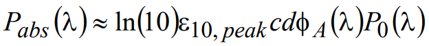
(11)
Next we consider a typical epifluorescence arrangement and determine P0(λ). In fluorescence microscopy the excitation light first passes through a train of optical components which direct and condition the light to provide maximum, uniform illumination of the field at the sample plane, then is transmitted by the exciter filter to provide out-of-band blocking, then is reflected by the dichroic beamsplitter, and finally is focused by the microscope objective onto the sample. Phenomenologically, following this reasoning one can write the incident power as
-equation-12.png?Status=Master&sfvrsn=d422eb5b_5)
(12)
where PL is the total power and L(λ) is the normalized spectral profile of the excitation light source, TX(λ) is the transmission spectrum of the exciter filter, RD(λ) is the reflectivity spectrum of the dichroic beamsplitter, and Ti(λ) is a factor introduced to account for the overall transmission of all other optics in the excitation light path (i.e. between light source and sample). The total power PL is further normalized by the integrated area under L(λ) and this mathematical treatment applies to all subsequent calculations. Therefore, the absorbed power at the sample can be written

(13)
Note that all of the wavelength dependent quantities are combined together on the right side of the above expression. To determine the total absorbed power Pabs,total (independent of wavelength), a simple integration over all wavelengths is performed:
(14)
Upon excitation, a fluorophore molecule emits fluorescence signal in all directions. Following from the above formalism describing the excitation path, the emitted fluorescence power that reaches the detector can be written as
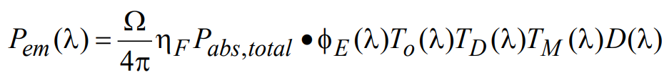
(15)
where Ω is the collection solid angle and can be determined from knowledge of the numerical aperture of the microscope objective used (see Appendix A), ηF is the quantum yield for fluorescence, Pabs,total is the absorbed light power (as calculated above), φE(λ) is the normalized spectral emission profile of the fluorophore, TD(λ) and TM(λ) are the transmission spectra of the dichroic and emission filters, respectively, D(λ) is the (dimensionless) detector response profile, and To(λ) is the combined transmission of all other optics in the emission path. For a CCD or CMOS camera, D(λ) can be assumed to be the wavelength dependent quantum efficiency, whereas for other types of detectors (for example, PMT) it is taken to be normalized detector responsivity. The total detected signal (denoted in the units of power), S, may then be calculated by integrating the emitted signal Pem(λ) over all wavelengths:
(16)
Having established a mathematical framework to calculate the detected fluorescence signal, S, built around an understanding of a simple fluorescence microscope, it is now possible to utilize the above approach to determine the excitation noise (NE) and fluorescence noise (NF) power levels.
Optical Noise Sources
There are two main sources of optical “noise” in a fluorescence microscope, namely: (i) excitation light noise, in the form of unblocked stray light; and (ii) background fluorescence that does not originate from desired fluorophores bound to desired targets. Background fluorescence can be further divided into two main types: autofluorescence from the sample and / or surrounding medium as well as other components in the system, like the microscope objective itself (hereafter referred to as “autofluorescence”), and fluorescence from the desired fluorophores that are not bound to the specific, intended targets of interest (referred to as “nonspecific binding”). Background fluorescence is typically the most problematic noise source to manage for many situations, whereas excitation light noise may be “designed out” of a carefully optimized optical system.
Excitation Light Noise
Unblocked stray light is a form of optical noise that originates from the excitation light source itself as well as the ambient light around the instrument, and does not originate from the sample or other sources of autofluorescence. Unblocked light from the excitation source can be a significant concern, since a large portion (several % or more) of the excitation light directed at the sample is reflected off of the microscope slide, cover slip, or other glass used to support the sample and directed back into the emission path. In an epifluorescence total-internal-reflection fluorescence (TIRF) microscope, nearly 100% of the laser excitation source is reflected off of the sample-glass interface and directed towards the emission path. Stray light from room lighting does not present a significant problem for confocal fluorescence microscopy, due to the fact that small diameter pinholes are used. However, this source of optical noise should be minimized in microscopy applications where pinholes are not used, such as in widefield and multiphoton microscopy. Optical noise originating from stray light reflections off of internal optics can be minimized through careful system design and the addition of beam dumps as necessary. In many imaging applications the level of stray light is reduced compared to background fluorescence noise and for most cases it can be considered as a constant value that can be empirically determined. However, for low concentrations of fluorophores, especially in applications such as single-molecule imaging, it can be significant and requires careful consideration, especially when choosing filters.
Since the most significant source of unblocked stray light noise is generally the excitation light source itself, here we estimate the size of this particular contribution to the overall optical noise. Following the formulism used above, the excitation light noise power (at the detector) can be written mathematically as

(17)
where fERφER(λ) is an empirical factor introduced to take into account the amount of reflected light that is redirected from the excitation path into the emission path (primarily by reflection off of the sample and its supporting glass). A typical value for fER might be ~ 0.04 (i.e., 4% reflection), thus representing the amount of light reflected from a clean glass microscope slide. However, this value is typically set higher to account for other specular reflections that occur from the sample and surrounding environment. Introducing the normalized wavelength dependent spectral reflectivity φER(λ) allows further flexibility in modeling the system behavior. The power of the total excitation light noise signal, NE, is calculated by integrating the wavelength-dependent power PE(λ) over all wavelengths:
(18)
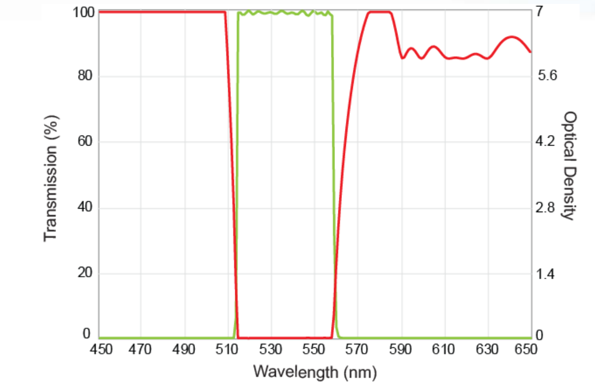
Figure 3: A plot of transmission (green) and blocking (red) characteristics for a common interference filter.
The blocking ability of thin-film interference filters is the primary weapon to prevent this reflected, stray light from reaching the detector. The filters work together in a complementary fashion so that the product of the filter spectra (particularly the exciter and emitter spectra) in the above equation should be very small at every wavelength at which the light source power and / or the detector response are appreciable. Filters with limited blocking capability lead to increased levels of stray excitation light reaching the detector and ultimately reduce image fidelity. Therefore, careful consideration is required to select the appropriate filters that spectrally select the desired light with high transmission and prevent out-of-band light by providing superior blocking with high optical density (OD) levels. An example of a high transmission and high blocking filter is shown in Figure 3.
Background Fluorescence Noise
Background fluorescence noise can result from autofluorescence as well as non-specific binding. Autofluorescence is generally understood as fluorescence originating from substances other than the target fluorophores of interest. Although often problematic, autofluorescence can be useful in the detection of biological species. Cells containing molecules such as pyridine (NAD, NADP) and flavin (FMN, FAD), which emit fluorescence photons when excited by UV or short-wavelength visible light, can serve as important diagnostic indicators. Useful information carried by autofluorescence originating from NADH can be used to monitor the metabolic state of living tissue. However, unless one is specifically looking for such signals, autofluorescence from these and other species is a problem that must be managed.
Sample autofluorescence comes from the surrounding environment in which the target portion of the sample is embedded. For the case of biological samples it typically results from the high density of organic molecules, such as NADH and flavins, that fluoresce under the same illumination conditions. It tends to be lower at longer wavelengths, and near-infrared (NIR) fluorophores have been developed to take advantage of this property. But this solution is not always suitable as many fluorophores with desirable biochemical properties are preferentially excited and imaged in the visible wavelength range. Alternative means to experimentally limit and prevent sample autofluorescence have been demonstrated. Recently Neumann and Gabel reported on reduction of sample autofluorescence observed in fluorescence imaging of aldehyde-fixed neural tissue. Their approach was to irradiate the tissue sample using a mercury arc lamp before staining [6]. By illuminating samples for approximately 20 minutes they found that all autofluorescence in the illuminated area could be eliminated. Although intriguing the approach of (pre-imaging) light dosing to reduce background autofluorescence is not always practical, especially for live cell imaging or for samples that are extremely sensitive to light induced damage.
Non-sample autofluorescence can come from any other element in the optical path through which the light propagates, such as the microscope objective, optical filters, and any other glass associated with the support of the sample. Generally filters utilize low-autofluorescence substrates to minimize this source of noise, but the glass types required to meet the demanding imaging performance of modern microscope objectives are more highly constrained, and thus there can be appreciable autofluorescence from the objective.
In many situations the most common result of autofluorescence is an undesirable and measurable increase in the light signal that is difficult to avoid and challenging to manage. The autofluorescence interferes with and obscures the detection of fluorescence emitted by the fluorophore of interest, making the detection of weak fluorescence signals difficult. Autofluorescence plagues single-channel fluorescence microscopy and requires careful consideration, especially when seeking quantitative results (e.g., in ratiometric imaging). For the case of multichannel imaging in dual-and triple-labeling experiments, it is critical to establish the level of background autofluorescence in each channel individually, as there can be significant differences in the levels of autofluorescence present in each channel.
Autofluorescence can be “removed” after an image is captured using spectral unmixing [7]. Spectral unmixing is a mathematical technique used to determine the quantities of specific component spectra from a measured spectrum that contains all of the components. It is most successful when the spectral signatures of the desired signal(s) as well as other, undesired light signals are known or can be accurately deduced from the measured data. The mathematical task is made more complicated and computationally challenging if unwanted background light signals are not well known nor easily determined.
Fluorescence noise resulting from non-specific binding is very straightforward to understand, although often challenging to eliminate. Sample preparation protocols must be optimized to minimize the amount of desired fluorophore molecules that do not chemically bind to the target species in the sample.
Well-executed control experiments can provide direct quantitative data that can be used to assess and differentiate between autofluorescence and non-specific binding contributions to the overall fluorescence signal. While time-consuming, this approach is important and worthwhile to follow, especially given that conditions typically change from experiment to experiment.
Modeling Autofluorescence and Non-specific Binding Noise Sources
Background fluorescence can be modeled as another spectral signal. Therefore, it is possible to use the same phenomenological model presented above to mathematically describe the detected background fluorescence noise, NF. As discussed above, this noise source can be broken into two basic components, so it is possible to treat autofluorescence noise (NAF) and non-specific binding noise (NNSB) independently.
Starting with autofluorescence noise (NAF), if the defining characteristics of the molecular species responsible for autofluorescence are known, then the absorbed power can be calculated as follows:

(19)
Here ε10,peak,AF represents the maximum value of the DMAC, and φA,AF(λ) is the normalized spectral absorption profile of autofluorescence. To determine the total absorbed power PAF,abs,total (independent of wavelength), a simple integration over all wavelengths is performed:
(20)
For autofluorescence noise, the wavelength-dependent power at the detector can now be written as

(21)
where ηAF is the quantum yield for autofluorescence and φE,AF(λ) is the autofluorescence normalized spectral emission profile. However, note that in practice quantum yield and spectral profile of sample autofluorescence might not be determined easily. But for a given sample the signal value of background autofluorescence as a percentage of the desired signal can be obtained from a control sample with no target fluorophore in the regime where the background is dominated by autofluorescence and excitation light noise is negligible. In this case ηAF and φE,AF(λ) may both be set equal to unity, and the empirical autofluorescence factor fAF in Eq. 21 is used to account for the relative strength of the autofluorescence with respect to the desired signal. All other terms in this equation are as defined previously. The total noise associated with autofluorescence NAF is then determined by integrating over all possible wavelengths:
(22)
Similarly, the wavelength-dependent power at the detector resulting from background fluorescence due to non-specific binding can be described mathematically as:

(23)
where all terms, including the empirical factor fNSB, are defined in an analogous fashion to those in the autofluorescence noise calculation above. The total noise signal associated with nonspecific binding fluorescence, NNSB, is then determined by integrating over all possible wavelengths:
(24)
In many cases the autofluorescence spectral profile is a broad, slowly varying function of wavelength, and as such one can simply model it as approximately constant over the bandwidth of the emission filter (as defined by TM(λ)). However, the spectral profile of fluorescence associated with non-specific binding tends to be strongly wavelength dependent since it is derived from established labeling fluorophores. When there is a single target fluorophore present, φNSB(λ) should be equivalent to φE(λ), the normalized spectral emission profile of the fluorophore. However, when there are multiple, known target fluorophores present, φNSB(λ) should be a properly weighted superposition of the associated spectra.
The total background fluorescence noise signal NF can now be written as

(25)
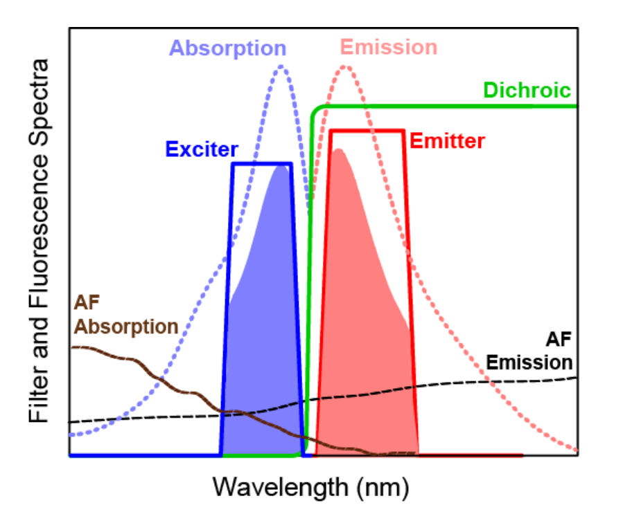
Figure 4: A schematic representation of example absorption and emission spectra for a target fluorophore, transmission spectra for a set of optical filters and absorption and emission spectra of autofluorescence (AF). For clarity, the spectral response profiles from the light source and detector have been omitted.
Practical Considerations for Managing Autofluorescence
As discussed above, there are numerous sources of background autofluorescence, including: microscope objectives and other internal optics in the light path, glass microscope cover slips or Petri dishes upon which most samples are mounted, mounting / fixing media, and even microscope immersion oil. The generation of fluorescence from microscope objectives is always undesirable but often unavoidable. The ideal microscope allows bright, high-contrast fluorescence observation using the minimum amount of excitation light in order to limit sample photodamage and fluorescence fading or photobleaching. However, most microscope objectives also generate autofluorescence under the same lighting conditions. One way to limit the level of autofluorescence is through the judicious choice of objectives manufactured from specially selected, non-fluorescing glasses that minimize artifacts arising from autofluorescence generated by internal lens elements. Many microscope manufacturers have developed specialized objectives that greatly reduce and limit autofluorescence for low-light imaging applications and it is important to seek their advice when considering specific fluorescence microscopy applications.
Microscope slides / cover slips upon which sample specimens are mounted also generate autofluorescence that is ultimately captured by the same collection optics (i.e., microscope objective) and transmitted to the detector. A wide variety of glass types exist such as, soda lime, borosilicate, and fused quartz (particularly useful when ultraviolet transparency is required). Reduced glass autofluorescence is achieved with of the removal of fluorescing impurities, such as metal oxide particles (e.g., ferric oxide). In addition, non-glass slides that exhibit reduced fluorescence are also available as alternatives. Permanox™ is an example of one such alternative. Permanox is a strong, biologically inert polymer material that is widely used for cell fixation and on-slide staining, and exhibits reduced autofluorescence across commonly used excitation wavelengths. However, one major drawback is that light transmission is approximately 70% at 400 nm compared to > 90% for many other glass types. Hence careful consideration is required given the amount of light that can be lost, especially if used in applications where the illumination light will first pass through the plastic substrate.
Another major problem encountered in fluorescence microscopy is the tendency of fluorophores to exhibit decreased fluorescence (fluorescence fading) or quench (due to the generation of free radicals) under light excitation. Because these effects are generally triggered by the fluorescing process itself, they are often called “photobleaching.” One way to overcome this problem is to use a mounting medium that not only reduces quenching but also fixes the specimen for imaging. However, the introduction of mounting media can also lead to increased levels of autofluorescence. Again, the origin of the autofluorescence signal is primarily due to the presence of (fluorescing) impurities present within the mounting medium. For example, glutaraldehyde works as a good fixative, but its use in fluorescence microscopy is limited due to intrinsically high levels of autofluorescence. An alternative is to use paraformaldehyde which exhibits low levels of autofluorescence. The simplest approach to understanding the level of autofluorescence generated by any mounting media – if not already quoted as part of the product specifications – is to perform control experiments. By applying a thin layer of mounting media to a clean glass / plastic cover slip one can record the photon counts associated with autofluorescence and determine a mean (constant) value over the image field of view.
Finally, immersion oil may also contribute to any autofluorescence signal. If immersion oil is required for imaging purposes then it is necessary to consider the spectral range of the excitation light. If the excitation ranges from about 400 – 800 nm immersion oil types A and B are most suitable. In order to understand whether or not a given type of immersion oil is nonfluorescing one must understand the manufacturer codes and designations, such as DF, HF, LF, etc. The simplest way to determine the level of autofluorescence generated under similar light excitation is to place a small amount of oil on a clean microscope slide, register the photon counts at the detector and determine the mean value. An example of the use of low autofluorescence immersion oil in fluorescence microscopy is shown in Figure 5 below.
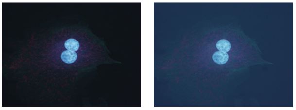
Figure 5: Improving image contrast in fluorescence microscopy: Fluorescence image of stained cells using low autofluorescence immersion oil (left) and general immersion oil. (Image courtesy of Olympus Corp.)
Conclusions
Understanding and managing the various contributions required to achieve high-fidelity fluorescence images in microscopy is challenging but critical. One must pay particular attention to the sources and relative levels of optical “noise.” Knowing how to best manage and control both excitation light noise and background fluorescence, and subsequently determine the true fluorescence signal is an art that is best practiced through experience. High-quality thin-film interference filters are the primary components responsible for ensuring negligible excitation light noise contribution. Fluorescence filters are also important for optimizing the level of the desired fluorescence signal relative to background fluorescence, to enable the brightest and highest-contrast fluorescence images.
References
[1] T. J. Fellers and M. W. Davidson, “CCD Noise Sources and Signal-to-Noise Ratio,” Molecular Expressions™ Optical Microscopy Primer: Digital Imaging in Optical Microscopy,micro.magnet.fsu.edu
[2] J. Joubert and D. Sharma, “Light Microscopy Digital Imaging,” Current Protocols in Cytometry, Unit 2.3, October, 2011.
[3] Handbook of Biological Confocal Microscopy, 3rd Ed., Edited by J. B. Pawley, Springer, 2006 (Chapters 4 and 12 and Appendix 3).
[4] Video Microscopy: The Fundamentals, S. Inoue and K. R. Spring, 2nd Ed., Plenum, New York, 1997.
[5] J.R. Lakowicz, Principles of Fluorescence Spectroscopy, 3rd Ed., Springer, 2006.
[6] M. Neumann and D. Gabel, “Simple Method for Reduction of Autofluorescence in Fluorescence Microscopy,” The Journal of Histochemistry and Cytochemistry, 50, (3), 437-439, 2002.
[7] J. R. Mansfield, K. W. Gossage, C. C. Hoyt, and R. M. Levenson, “Autofluorescence removal, multiplexing, and automated analysis methods for in-vivo fluorescence imaging,” Journal of Biomedical Optics, 10, (4), 041207, 2005.
Authors
Neil Anderson, Ph.D., Prashant Prabhat, Ph.D. and Turan Erdogan, Ph.D.
Appendix A: Concept of Solid Angle in Imaging Microscopy
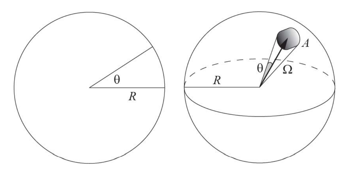
Figure A1: Illustration of the analogy between angles and solid angles.
Solid angles in three dimensions (3D) are analogous to simple angles in 2D (see figure A1). In 2D, an angle θ measured in radians is the length of an arc on a unit circle (radius R of 1 unit) that is subtended by the angle. The entire circumference has a radian measure of 2π. Similarly, in 3D, a solid angle Ω measured in steradians is the area A of the surface patch on a unit sphere (radius R of 1 unit) subtended by the solid angle.
Mathematically, the solid angle associated with an area on a sphere of radius R can be computed using
To relate the solid angle to the half angle θ of the cone with which it is associated, consider the diagram shown in Figure A1 (right). The area A is given by
Therefore, the solid angle Ω is
Recognizing that the cone may represent the collection geometry of a microscope objective, it is possible to calculate the solid angle of light collection associated with a particular objective. The numerical aperture (NA) of a microscope objective is defined in terms of the half-angle θ as
where n is the refractive index of the medium through which the light is collected (generally air, water, or index-matching oil). Then the solid angle Ω associated with a particular microscope objective is given by
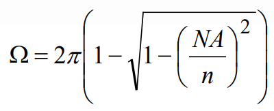
For example, an air objective with an NA of 0.7 collects light over a solid angle of Ω=1.8 steradians, whereas an oil-immersion objective with an NA of 1.4 collects light over a solid angle of Ω=3.8 steradians. The air objective collects about 14% of the isotropically emitted fluorescence, whereas the high-NA oil-immersion objective collects over 30% of the fluorescence.
Appendix B: List of variables and expected range of values
| Symbol | Unit | Range of Value | Description |
| ρ | molecules/cm3 | ≥ 0 | number density of target fluorophore molecules |
| ε(λ) | cm2/mole = M–1cm–1 | ≥ 0 | extinction coefficient of target fluorophore |
| ε10(λ) | cm2/mole = M–1cm–1 | ≥ 0 | decadic molar extinction coefficient (or decadic molar absorption coefficient, DMAC) of target fluorophore |
| ε10,peak | cm2/mole = M–1cm–1 | ≥ 0 | maximum value of the decadic molar extinction coefficient of target fluorophore |
| ε10,peak,AF | cm2/mole = M–1cm–1 | ≥ 0 | maximum value of the decadic molar extinction coefficient of autofluorescence |
| φΑ(λ) | dimensionless | [0,1] | normalized spectral absorption profile of the target fluorophore |
| φΑ AF(λ) | dimensionless | [0,1] | autofluorescence normalized spectral absorption profile |
| φE(λ) | dimensionless | [0,1] | normalized spectral emission profile of the target fluorophore |
| φE,AF(λ) | dimensionless | [0,1] | autofluorescence normalized spectral emission profile |
| φER(λ) | dimensionless | [0,1] | normalized spectral profile of reflected light that is redirected from the excitation path into the emission path (primarily by reflection off of the sample and its supporting glass) |
| φNSB(λ) | dimensionless | [0,1] | normalized spectral profile of non-specific binding |
| ηF | dimensionless | [0,1] | quantum yield for target fluorophore |
| ηAF | dimensionless | [0,1] | quantum yield for autofluorescence |
| ηNSB | dimensionless | [0,1] | quantum yield for non-specific binding |
| θ | dimensionless | [0, π/2] | half cone angle of the microscope objective |
| σ(λ) | cm2 | ≥ 0 | molecular absorption cross-section |
| Ω | steradian | [0, 4π] | collection solid-angle and can be determined from knowledge of the numerical aperture of the microscope objective used (see Appendix-A) |
| c | M = molar = moles / liter = 10–3 moles / cm3 | ≥ 0 | molar concentration of target fluorophore |
| cAF | M = molar = moles / liter = 10–3 moles / cm3 | ≥ 0 | molar concentration of autofluorescence |
| d | cm | ≥ 0 | thickness of a slab of fluorophore |
| fAF | dimensionless | [0,1] | an empirical factor introduced to take into account the relative strength of autofluorescence signal |
| fER | dimensionless | [0,1] | an empirical factor introduced to take into account the amount of reflected light that is redirected from the excitation path into the emission path (primarily by reflection off of the sample and its supporting glass). |
| fNSB | dimensionless | [0,1] | an empirical factor introduced to take into account the relative strength of signal from non-specific binding |
| n | dimensionless | ≥ 1 | refractive index of the medium through which the light is collected (generally air, water, or index-matching oil) |
| A | cm2 | ≥ 0 | area on the surface of a sphere of radius R, subtending solid angle Ω at the center (see Appendix-A) |
| D(λ) | dimensionless | [0,1] | detector spectral response profile (nonnormalized when denoting quantum efficiency of a CCD or CMOS detector and normalized when denoting other detector responsivities) |
| L(λ) | dimensionless | [0,1] | normalized spectral profile of the excitation light source |
| N | dimensionless | 6.022x10²³ | Avogadro’s number |
| NAF | mW | ≥ 0 | total noise signal associated with autofluorescence |
| NE | mW | ≥ 0 | excitation light noise |
| NF | mW | ≥ 0 | fluorescence noise (for example, autofluorescence and non-specific binding) |
| NNSB | mW | ≥ 0 | total noise signal associated with nonspecific binding fluorescence |
| NT | mW | ≥ 0 | the total (undesired) optical noise |
| NA | dimensionless | ≥ 0 | numerical aperture of a microscope objective |
| Pabs(λ) | mW | ≥ 0 | absorbed power by target fluorophore |
| Pabs,total(λ) | mW | ≥ 0 | total absorbed power by target fluorophore (independent of wavelength) |
| PAF,abs(λ) | mW | ≥ 0 | absorbed power by autofluorescence |
| PAF,abs,total(λ) | mW | ≥ 0 | total absorbed power by autofluorescence (independent of wavelength) |
| Pd(λ) | mW | ≥ 0 | power of light emerging from a slab of thickness d |
| PE(λ) | mW | ≥ 0 | power of excitation light noise |
| Pem(λ) | mW | ≥ 0 | emitted fluorescence power that reaches the detector |
| PL | mW | ≥ 0 | total power of the excitation light source |
| PNSB(λ) | mW | ≥ 0 | emission power from non-specific binding |
| P0(λ) | mW | ≥ 0 | power of the incident light at sample |
| R | cm | ≥ 0 | radius of sphere (see Appendix-A) |
| RD(λ) | dimensionless | [0,1] | reflectivity spectrum of the dichroic beamsplitter (non-normalized) |
| S | mW | ≥ 0 | total emitted (desired) fluorescence signal |
| SNR | dimensionless | ≥ 0 | signal-to-noise ratio |
| Ti(λ) | dimensionless | [0,1] | transmission spectrum of all other optics in the excitation light path (non-normalized) |
| TX(λ) | dimensionless | [0,1] | transmission spectrum of the exciter filter (non-normalized) |
| TD(λ) | dimensionless | [0,1] | transmission spectrum of the dichroic (non-normalized) |
| TM(λ) | dimensionless | [0,1] | transmission spectrum of the emission filters (non-normalized) |
| T0(λ) | dimensionless | [0,1] | combined transmission spectrum of all other optics in the emission path (nonnormalized) |